ReLightGS: Relighting Existing 3D Gaussian Splatting Scenes Without Retraining

Abstract

3D Gaussian Splatting (3DGS) enables high-quality real-time novel-view synthesis, but standard trained Gaussian scenes provide little control over illumination. Their learned appearance entangles lighting and material appearance, making existing scenes difficult to relight without the original training images or additional optimization.

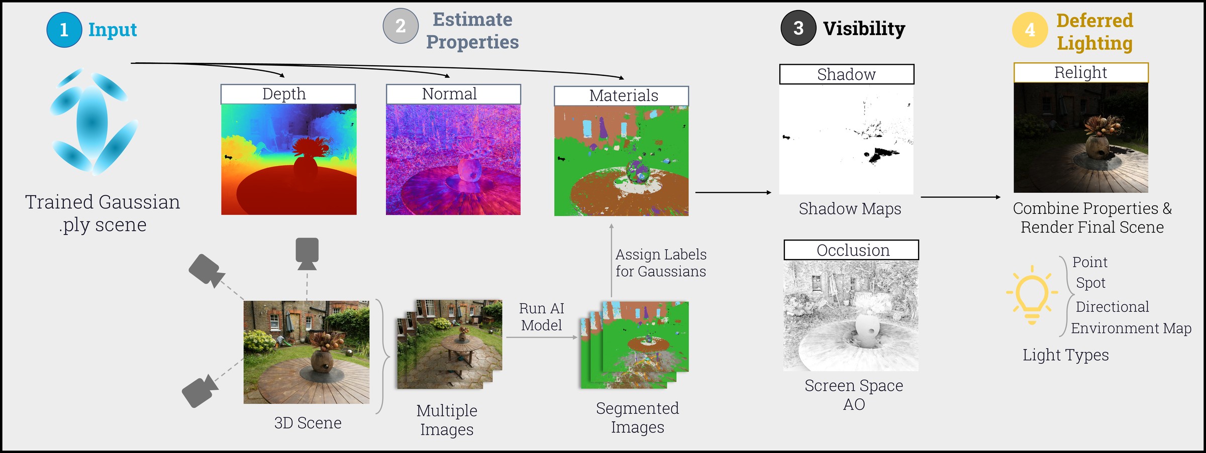
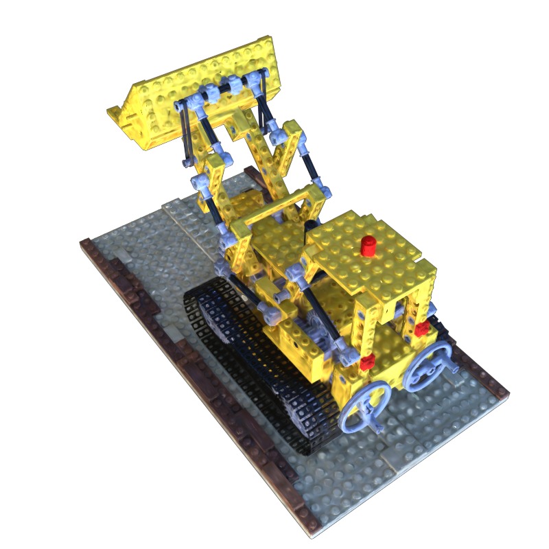
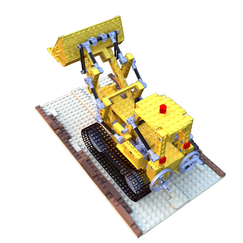
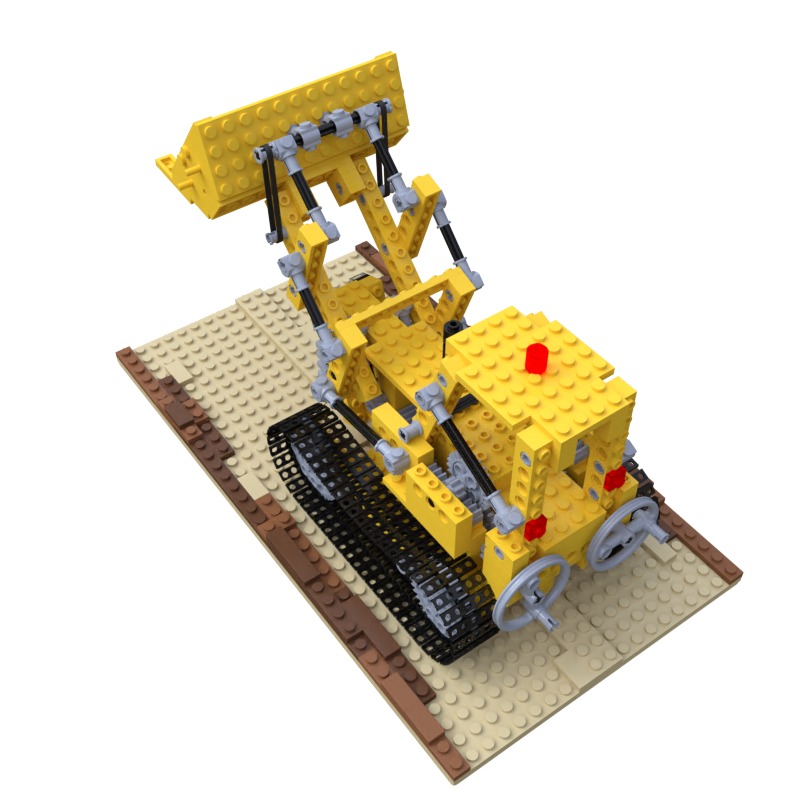
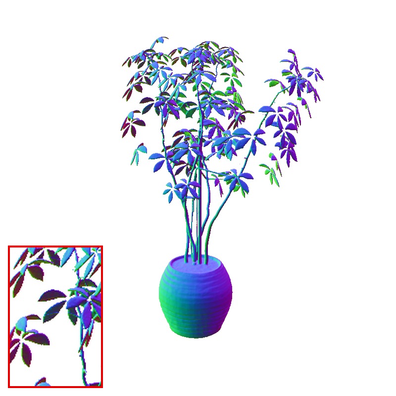
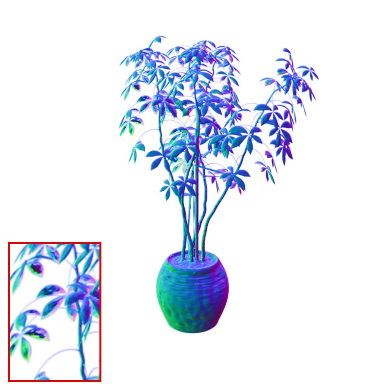
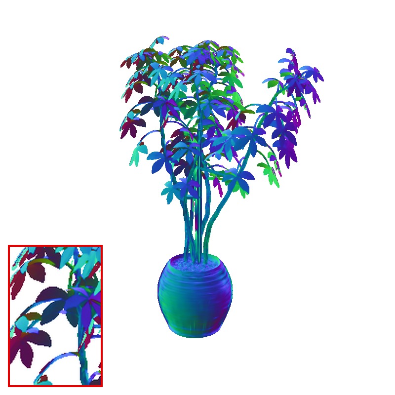
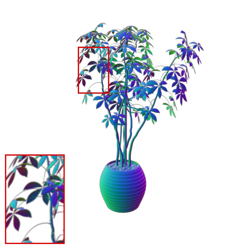
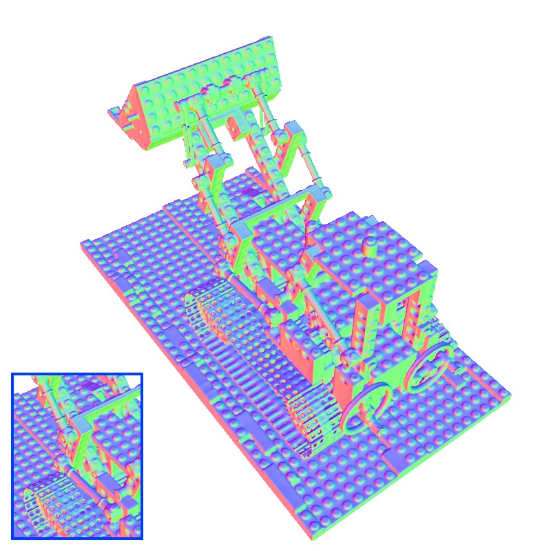
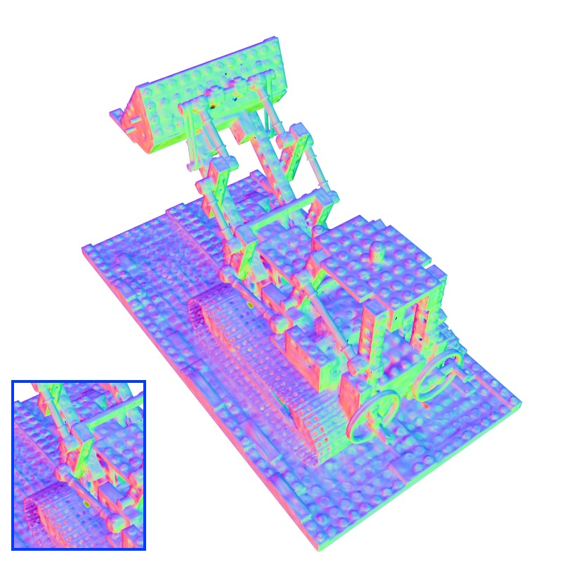
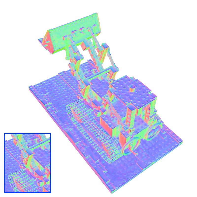
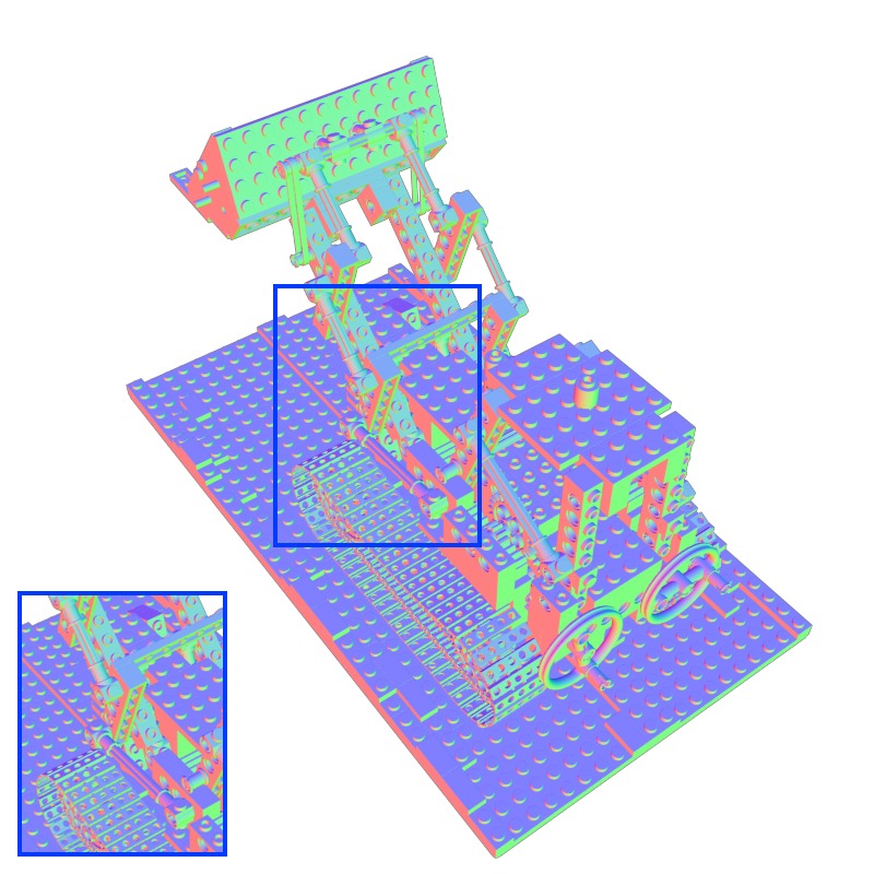
We propose ReLightGS, a deferred relighting pipeline for already trained 3DGS scenes that operates directly on fixed exported Gaussian models, without access to the images used to train them and without further retraining. The method constructs a Gaussian G-buffer, reconstructs approximate depth and normals, assigns PBR material parameters from lifted material labels, and computes illumination with approximate visibility and occlusion. Using pretrained vanilla 3DGS scenes from the TensoIR Synthetic dataset as input, we evaluate our method under multiple HDR environment maps and compare the results with inverse-rendering baselines. Our evaluation demonstrates that our approach allows plausible relighting without retraining, although baked illumination and approximate geometry remain limitations.

Video

Method Overview

Our method pipeline: from a fixed Gaussian scene to a relit image.

Results

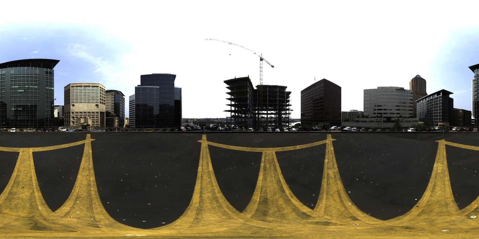
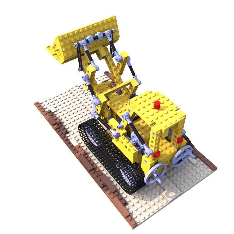
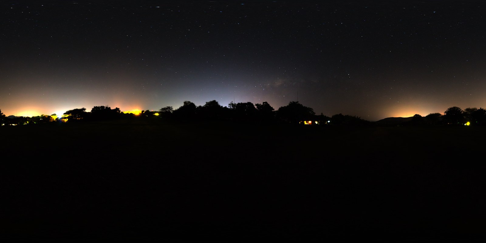
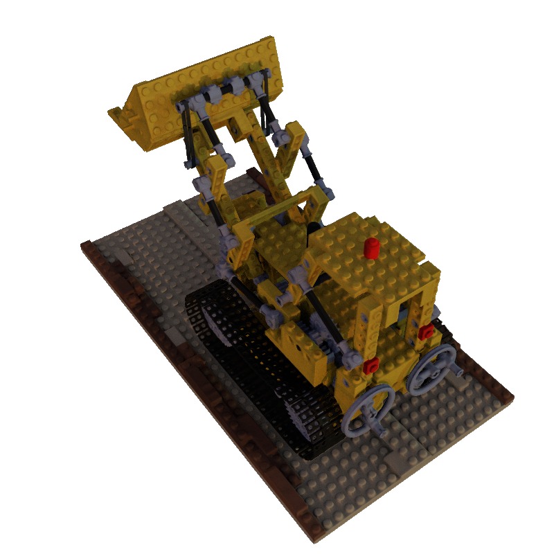
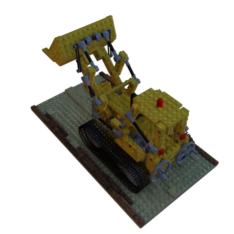
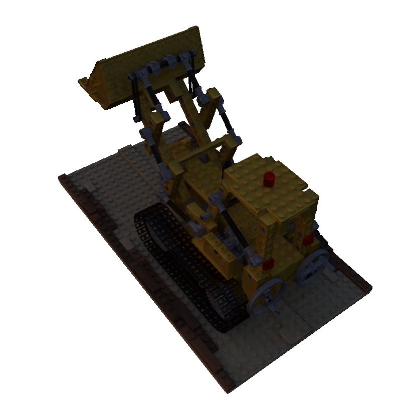
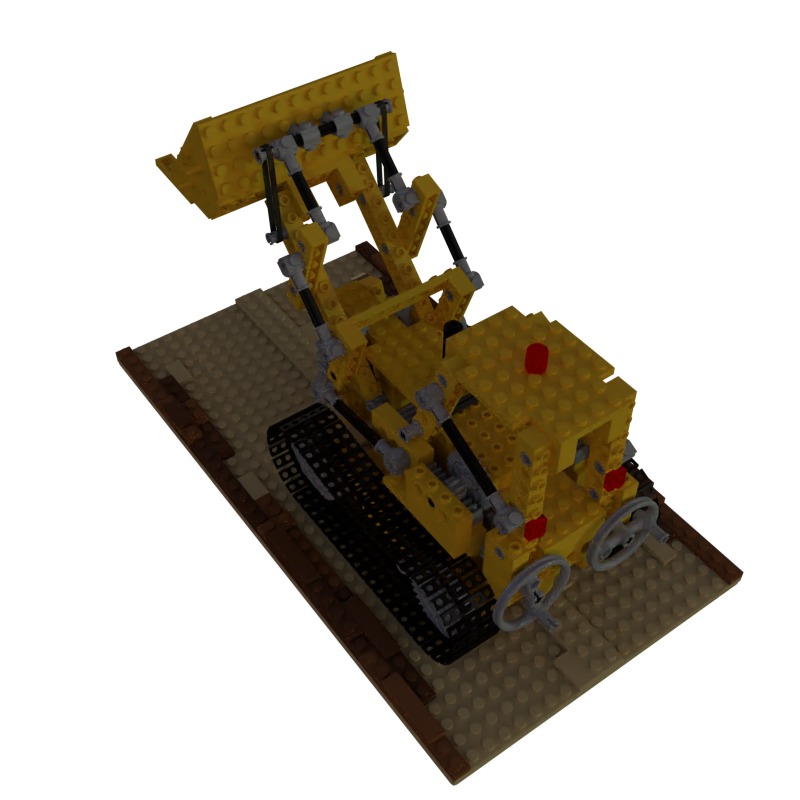
We evaluate on the four object-centric TensoIR Synthetic scenes (armadillo, ficus, hotdog, lego), with relighting metrics averaged over five HDR environment maps (bridge, city, fireplace, forest, night). The scenes are vanilla 3DGS models trained for 30,000 iterations, and baseline numbers are adapted from the GS-IR evaluation. For this environment-map benchmark the map intensity is set to 5.0, and screen-space ambient occlusion and shadow mapping are disabled, since it uses only environment lighting. Despite operating post-hoc on a fixed vanilla 3DGS representation, with no access to the original images and no retraining, ReLightGS improves over the Gaussian-based GS-IR baseline on every metric.

	Method	Normal MAE↓	Relight
	Method	Normal MAE↓	PSNR↑	SSIM↑	LPIPS↓
Neural field based rendering	NeRFactor	6.314	23.383	0.908	0.131
	InvRender	5.074	23.973	0.901	0.101
	NVDiffrec	6.078	19.880	0.879	0.104
	TensoIR	4.100	28.580	0.944	0.081
Gaussian splat based rendering	GS-IR	4.948	24.374	0.885	0.096
Gaussian splat based rendering	Ours	4.780	25.920	0.906	0.095

Quantitative comparison on the TensoIR Synthetic dataset. Cells are shaded by per-column rank (salmon = best, white = worst). Baseline results are adapted from GS-IR; relighting metrics are averaged over five HDR environment maps (bridge, city, fireplace, forest, night).

All four scenes relit under a city environment, produced directly from the fixed Gaussian models.

Normals reconstructed directly from the fixed Gaussian geometry for the armadillo, ficus, hotdog, and lego scenes.

TensoIR

GS-IR

Ours

GT

City HDR environment map — Lego
(City Env)

Night HDR environment map — Lego
(Night Env)

TensoIR

GS-IR

Ours

GT

Ficus (normals)

Lego (normals)

References

[Kerbl 2023] Kerbl, B., Kopanas, G., Leimkühler, T. and Drettakis, G., 2023. 3D Gaussian Splatting for Real-Time Radiance Field Rendering. ACM Transactions on Graphics (TOG), 42(4).

[Liang 2024] Liang, Z., Zhang, Q., Feng, Y., Shan, Y. and Jia, K., 2024. GS-IR: 3D Gaussian Splatting for Inverse Rendering. CVPR, pp.21644-21653.

[Jin 2023] Jin, H., Liu, I., Xu, P., Zhang, X., Han, S., Bi, S., Zhou, X., Xu, Z. and Su, H., 2023. TensoIR: Tensorial Inverse Rendering. CVPR, pp.165-174.

[Zhang 2021] Zhang, X., Srinivasan, P.P., Deng, B., Debevec, P., Freeman, W.T. and Barron, J.T., 2021. NeRFactor: Neural Factorization of Shape and Reflectance under an Unknown Illumination. ACM Transactions on Graphics (TOG), 40(6).

[Zhang 2022] Zhang, Y., Sun, J., He, X., Fu, H., Jia, R. and Zhou, X., 2022. Modeling Indirect Illumination for Inverse Rendering (InvRender). CVPR, pp.18643-18652.

[Munkberg 2022] Munkberg, J., Hasselgren, J., Shen, T., Gao, J., Chen, W., Evans, A., Müller, T. and Fidler, S., 2022. Extracting Triangular 3D Models, Materials, and Lighting From Images (NVDiffrec). CVPR, pp.8280-8290.

[Zhang 2026] Zhang, B., Fang, C., Shrestha, R., Liang, Y., Long, X. and Tan, P., 2026. RaDe-GS: Rasterizing Depth in Gaussian Splatting. ACM Transactions on Graphics (TOG), 45(2).

[Kheradmand 2025] Kheradmand, S., Vicini, D., Kopanas, G., Lagun, D., Yi, K.M., Matthews, M. and Tagliasacchi, A., 2025. StochasticSplats: Stochastic Rasterization for Sorting-Free 3D Gaussian Splatting. ICCV, pp.26326-26335.

[Upchurch 2022] Upchurch, P. and Niu, R., 2022. A Dense Material Segmentation Dataset for Indoor and Outdoor Scene Parsing. ECCV, pp.450-466.

[Mittring 2007] Mittring, M., 2007. Finding Next Gen: CryEngine 2. ACM SIGGRAPH 2007 Courses, pp.97-121.

[Gao 2024] Gao, S., 2024. 3DGS.cpp: High Performance 3D Gaussian Splatting with Vulkan.

[NVIDIA] NVIDIA. vk_gaussian_splatting: Lighting, Shading and Shadows.